Linear Systems and Quadratic Extrema   

Many applications involve quadratic functions, where a quadratic function is a function that is a second degree polynomial in each variable. When a quadratic function has a critical point, it must be the solution to a system of simultaneous linear equations (also known as a linear system) of the form

ax + by  =  r cx + dy  =  s

One way of solving a linear system is to multiply the first equation by -c, multiply the second equation by a, and combine the two equations to eliminate x:

-acx - bcy  =  -r c   acx +  ady  =  s a ( ad-bc) y  = sa-rc

After solving for y, substitution can be used to determine x.  Or any of a number of other variations may be used instead.       

EXAMPLE 4    Find the point(s) on the plane z = x+y-3 that are closest to the origin.

Solution: To begin with, we let f denote the square of the distance from a point ( x,y,z) to the origin. Consequently,

f = x2 + y2 + z2

Substituting z = x+y-3 thus yields

f( x,y) = x2 + y2 + (x+y-3)2

Since f_x = 4x+2y-6 and   f_y = 2x+4y-6, we must solve

4x+2y = 6,        2x+4y = 6

Multiplying the second equation by -2 yields

4x + 2y = 6 -4x - 8y = -12 0x -6y   = -6

so that y = 1. Similarly, we find that x = 1, so the critical point is ( 1,1) . Moreover, f_xx = 4, f_xy = 2, and f_yy = 4, so that the discriminant is

D = fxx fyy - fxy2 = 16 - 4 = 12 > 0

Thus, every "slice'' is concave up and correspondingly, f has a minimum at ( 1,1) . Substitution yields

z = 1+1-3 = -1

so that ( 1,1,-1) is the point in the plane z = x+y-3 that is closest to the origin.      

One of the most important applications in statistics is finding the equation of the line that best fits a data set of the form

( x1,y1) ,( x2,y2) ,¼,(xn,yn)

where by best fit we mean the line which produces the least error. Specifically, the j^th error or residual in approximating the data set with the line y = mx+b is

ej = mxj+b-yj

Thus, e_j² is the square of the vertical distance from the point to the line.

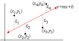
We then define the least squares line for the data set to be the line with the slope m and the y-intercept b that minimizes the total squared error

E( m,b) = n å j = 1  ( mxj+b-yj) 2

That is, the least squares line minimizes the sum of the squares of the residuals.       

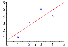
EXAMPLE 6    Find the least squares line for the data set (1,1),  ( 2,3),  ( 3,5), and (4,4) .       

Solution: To find E( m,b) , we calculate the squares of the residuals for each of the data points and then compute their sum:

e12: ( m·1+b-1)2 =   m2+2mb-2m+b2-2b+1 e22: ( m·2+b-3)2 = 4m2+4mb-12m+b2-6b+9 e32: ( m·3+b-5)2 = 9m2+6mb-30m+b2-10b+25 e42: ( m·4+b-4)2 = 16m2+8mb-32m+b2-8b+16 E( m,b) = 30m2+20mb-76m+4b2-26b+51

The first partial derivative of E( m,b) are

Em( m,b) = 60m+20b-76    and    Eb( m,b) = 20m+8b-26

Thus, the critical points must satisfy

60m+20b  =  76 20m+8b  =  26

Multiplying the latter by -3 yields

60m + 20b  =    76 -60m - 24b  =   -78 0m -   4b  =   -2

Thus, b = 0.5 and likewise, we find that m = 1.1.
        The second derivatives of E( m,b) are

Emm = 60,    Emb = 20,    Ebb = 8

and as a result, the discriminant is

D = 60·8-( 20) 2 = 80 > 0

which implies that E( m,b) has a minimum at m = 1.1 and b = 0.5. Thus, the least squares line for the data set ( 1,1) , ( 2,3) , ( 3,5) , and ( 1,4) is y = 1.1x+0.5:

Typically, due to the size of the data sets involved, least squares problems are not solved by hand.  Correspondingly, our investigation of least squares problem is treated with greater depth and more examples in the associated Maple worksheet.