Scalar Fields
Often functions of 2 variables are interpreted to be scalar
fields, where a scalar field is the assignment of a scalar to each point in
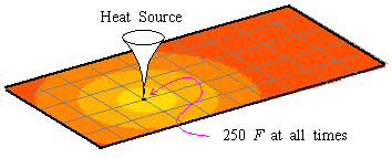
the plane. For example, let's suppose that a 10˘˘×5˘˘ rectangular plate is at room temperature of 70°F when a heat source at a temperature of 250°F is applied at a
point 3˘˘ from a shorter side and 2˘˘ from
a longer side of the plate (i.e., at the point ( 3,2) if ( 0,0) is at a corner).

Suppose now that 5 seconds after the heat source is applied, each point ( x,y) on the plate's surface then has a unique temperature, T = g( x,y) where
|
g( x,y) = 70+180e-( x-3) 2/10-( y-2)2/10 |
| (1) |
That is, g( x,y) is the scalar field which maps a point ( x,y) to the temperature T of the surface at that point
after 5 seconds.
It follows that the temperature at the origin is
|
T = 70+180e-( 0-3) 2/10-( 0-2) 2/10 = 119°F |
|
and that the temperature at the point ( 1,1) is
|
T = 70+180e-( 1-3) 2/10-( 1-2) 2/10 = 179°F |
|
Temperatures at all integer pairs ( x,y) in [0,10] ×[ 0,5] are shown below:
If we now compute the gradient of g, we obtain
|
Ńg = 180e-( x-3) 2/10-( y-2)2/10 |

|
- |
1
5
|
x+ |
3
5
|
,- |
1
5
|
y+ |
2
5
|  |
|
| (3) |
At the point ( 1,1) , we then have
|
|
|
|
180e-( 1-3) 2/10-( 1-2)2/10 |

|
- |
1
5
|
+ |
3
5
|
,- |
1
5
|
+ |
2
5
|  |
|
| |
|
| |
|
|
|
This defines the direction in which the temperature is increasing the
fastest. Moreover,
|
Dug = ||
á 43.668,21.834
ñ || = 48. 82°F per inch |
|
is the rate of increase in the direction of fastest increase.
Level curves of scalar fields are often referred to using prefixes such as
``iso-'' or ``equi-''. For example, the level curves of a scalar temperature
field are known as isotherms. Below are shown the isotherms of the
temperature field (1) for temperatures 179°F, 217°F, and 233°F
We'll explore more applications of scalar fields in the exercises.

